Pyplatefit tutorial¶

Pyplatefit tutorial

Roland Bacon

Introduction¶

Pyplatefit is a python module to perform emission line fitting of astronomical spectra. Although it has been developed for the MUSE integral field spectrograph, it should work for spectrum delivered by other instruments, provided that the input spectrum is in MPDAF format.

The program take as input a spectrum and an input redshift and return the list of emission lines parameters: e.g. flux, velocity dispersion, equivalent width and their errors. The program perform a continuum fit, using a simple population model and then fit the emission lines after continuum subtraction. In addition the program can also perform basic absorption lines fit.

Lines are organized into families. All lines from the same family share the same velocity (or redshift) and velocity dispersion. In addition to the two Balmer and Forbidden families, resonnant lines like \({\rm Ly\alpha}\) or \({\rm Mg_{II}}\) are fitted separately as distinct families. Absorption lines are also processed as a separate family. Each family is fitted independantly.

All emission (and absorption) lines are modelled as Gaussians with 3 parameters: velocity, velocity dispersion (in \({\rm km s^{-1}}\)) and flux. The only exception, is the \({\rm Ly\alpha}\) line which is fitted as a skewed Gaussian, with an additional \({\rm \gamma}\) parameter measing the asymetry of the line.

\[{\rm F(\lambda) = F_{max} \left[ 1 + erf \left( \gamma \frac{\left(\lambda - \lambda_{0}\right)}{\sqrt 2 \sigma} \right) \right] \left[ exp \left( - \frac{\left(\lambda - \lambda_{0}\right)^2}{2 \sigma^2} \right) \right] }\]

Optionnaly, double peaked \({\rm Ly\alpha}\) line can be fitted as the sum of two skewed Gaussians.

The program use the front-end lmfit minimization package based on scipy optimize non-linear least-squares minimization. The default minimization routine is the Trust Region Reflective least squares algorithm, which is more robust and gives better estimate error estimate than the classical Levenberg–Marquardt algorithm. Other minimization algorithm can be selected, see lmfit documentation for detail. The MCMC emcee package is also used to improve error computation.

Importing modules¶

[1]:

%matplotlib inline
import matplotlib.pyplot as plt
import os
import mpdaf, pyplatefit
from mpdaf.obj import Spectrum
from pyplatefit import fit_spec, plot_fit, print_res
print(f"MPDAF version {mpdaf.__version__}")
print(f"Pyplatefit version {pyplatefit.__version__}")

MPDAF version 3.6.dev21+g8acab809
Pyplatefit version 0.8.dev0+g02018a5.d20220511

Basic usage¶

Input data¶

The input spectrum must be in MPDAF format, ie with proper wcs information and data and variance extensions. See MPDAF documentation for more detailed information. The input redshift z (in vacuum) must be precise enough. Pyplatefit will refine it but cannot deal with poorly known redshift.

[2]:

datadir = '../tests/test_data'
sp = Spectrum(os.path.join(datadir, 'udf10_00002.fits'))
sp.info()

[INFO] 3681 Spectrum (../tests/test_data/udf10_00002.fits)
[INFO] .data(3681) (1e-20 erg / (Angstrom cm2 s)), .var(3681)
[INFO] wavelength: min:4750.00 max:9350.00 step:1.25 Angstrom

Running the minimisation¶

fit_spec is the main routine, see later for the meaning of all input parameters.

[3]:

res = fit_spec(sp, z=0.41892)

[DEBUG] Fit continuum
[DEBUG] Fit emission lines
[DEBUG] Preparing data for fit
[DEBUG] Getting lines from default line table...
[DEBUG] 21.3 % of the spectrum is used for fitting.
[DEBUG] Initialize fit
[DEBUG] Found 2 non resonnant line families to fit
[DEBUG] Init Fit of family balmer
[DEBUG] Found 9 lines to fit
[DEBUG] added 9 gaussian to the fit
[DEBUG] Init Fit of family forbidden
[DEBUG] Found 13 lines to fit
[DEBUG] added 13 gaussian to the fit
[DEBUG] Found 0 resonnant line families to fit
[DEBUG] Fitting of Line Family: balmer
[DEBUG] Lmfit fitting: {'method': 'least_square', 'xtol': 0.001}
[DEBUG] `xtol` termination condition is satisfied. after 7 iterations, reached minimum = 192511.056 and redChi2 = 249.367
[DEBUG] Fitting of Line Family: forbidden
[DEBUG] Lmfit fitting: {'method': 'least_square', 'xtol': 0.001}
[DEBUG] `xtol` termination condition is satisfied. after 9 iterations, reached minimum = 196213.255 and redChi2 = 255.486
[DEBUG] Saving balmer results to tablines and ztab
[DEBUG] Saving forbidden results to tablines and ztab

By default the logging is in DEBUG mode, but it is possible to run it in quiet mode, using the python logging module.

[4]:

import logging
logger = logging.getLogger('pyplatefit')
logger.setLevel('INFO')
res = fit_spec(sp, z=0.41892)
logger.setLevel('DEBUG')

Analysis of result¶

The program return a python dictionary with a following items:

ztable: the redshift table (astropy format)
lines: the lines table (astropy format)
spec_fit: the fitted spectrum (MPDAF format)

Note that the resulting dictionary include many other items. We describe here only the ones relevant for this basic usage. More is given later in the advanced usage section.

The ztable contain global information for each fitted family.

[5]:

res['ztable']

[5]:

Table length=2

FAMILY	VEL	VEL_ERR	Z	Z_ERR	Z_INIT	VDISP	VDISP_ERR	LINE	SNRMAX	SNRSUM	SNRSUM_CLIPPED	NL	NL_CLIPPED	RCHI2	NFEV	STATUS	METHOD
str20	float64	float64	float64	float64	float64	float64	float64	str20	float64	float64	float64	int64	int64	float64	int64	int64	str25
balmer	82.13	3.86	0.41931	1.83e-05	0.41892	66.11	4.26	HBETA	20.62	13.28	12.98	9	5	249.37	7	3	least_squares
forbidden	92.49	5.29	0.41936	2.50e-05	0.41892	66.65	6.07	OII3727b	17.26	16.86	20.72	12	5	255.49	9	3	least_squares

In this case the fit converge to similar velocity (VEL) and velocity dispersion (VDISP) for the balmer and forbidden lines. The highest SNRMAX and corresponding LINE are reported. The number of fitted lines before (NL) and after SNR>3 clipping (NL_CLIPPED) are also given. An relevant parameter is the SNR sum of the clipped lines (SNRSUM_CLIPPED). The convergence status (STATUS), number of function evaluation (NFEV), reduced \(\chi^2\) (RCHI2) and name of the algorithm (METHOD) are also given. Codification of convergence status is specific for each method, for the default least_squares (Trust Reflective Least Square) method see the scipy documentation. When convergence is achieved we expect to get status=3, and status=0 if the algorithm did not converge in the maximum of iterations.

The detailed information for each fitted lines is given in the lines table. In the following we list the five highest SNR emission lines, excluding the blended lines (e.g OII3727b = OII3726+OII3729).

[6]:

lines = res['lines'].copy()
lines = lines[~lines['ISBLEND']]
lines.sort('SNR')
lines[::-1][0:5]

[6]:

Table length=5

FAMILY	LINE	ISBLEND	LBDA_REST	DNAME	VEL	VEL_ERR	Z	Z_ERR	Z_INIT	VDINST	VDISP	VDISP_ERR	FLUX	FLUX_ERR	SNR	SKEW	SKEW_ERR	LBDA_OBS	PEAK_OBS	LBDA_LEFT	LBDA_RIGHT	FWHM_OBS	NSTD	LBDA_LNSTD	LBDA_RNSTD	BLEND	EQW	EQW_ERR	CONT_OBS	CONT	CONT_ERR
str20	str20	bool	float64	str20	float64	float64	float64	float64	float64	float64	float64	float64	float64	float64	float64	float64	float64	float64	float64	float64	float64	float64	float64	float64	float64	int64	float64	float64	float64	float64	float64
balmer	HBETA	False	4862.68	Hβ	82.13	3.86	0.41931	1.83e-05	0.41892	42.93	66.11	4.26	8567.47	415.43	20.62	0.00	0.00	6899.74	1884.01	6897.60	6901.87	4.27	-2.19	6893.33	6906.15	0	-7.86	0.40	768.17	1089.98	30.89
forbidden	OII3729	False	3729.88	[Oɪɪ]	92.49	5.29	0.41936	2.50e-05	0.41892	61.97	66.65	6.07	6065.85	435.24	13.94	0.00	0.00	5292.56	1506.24	5290.67	5294.45	3.78	-2.44	5282.93	5298.23	3727	-7.20	0.55	593.92	842.73	42.22
forbidden	NII6584	False	6585.28	None	92.49	5.29	0.41936	2.50e-05	0.41892	33.19	66.65	6.07	11604.35	1017.52	11.40	0.00	0.00	9344.30	1994.89	9341.57	9347.03	5.47	-1.79	9336.10	9352.50	0	-11.65	1.45	701.99	996.06	292.68
balmer	HGAMMA	False	4341.68	Hγ	82.13	3.86	0.41931	1.83e-05	0.41892	49.80	66.11	4.26	3647.94	348.92	10.45	0.00	0.00	6160.48	855.67	6158.47	6162.48	4.01	-1.85	6154.47	6166.49	0	-3.28	0.32	784.02	1112.46	36.08
forbidden	OII3726	False	3727.09	None	92.49	5.29	0.41936	2.50e-05	0.41892	62.04	66.65	6.07	4340.88	426.09	10.19	0.00	0.00	5288.60	1078.16	5286.71	5290.49	3.78	-2.44	5282.93	5298.23	3727	-5.19	0.53	589.73	836.78	41.88

The detailed explanation of all columns is given in appendix. Note that parameters (unless specfified by OBS in the column name) are given in rest frame. Velocity dispersion (VDISP) is corrected for MUSE instrumental resolution.

A visual check can be performed with the plot_fit routine.

[7]:

fig,ax = plt.subplots(1,3,figsize=(20,5))
plot_fit(ax[0], res)
plot_fit(ax[1], res, line='OII3729')
plot_fit(ax[2], res, line='OII3729', line_only=True, margin=20)

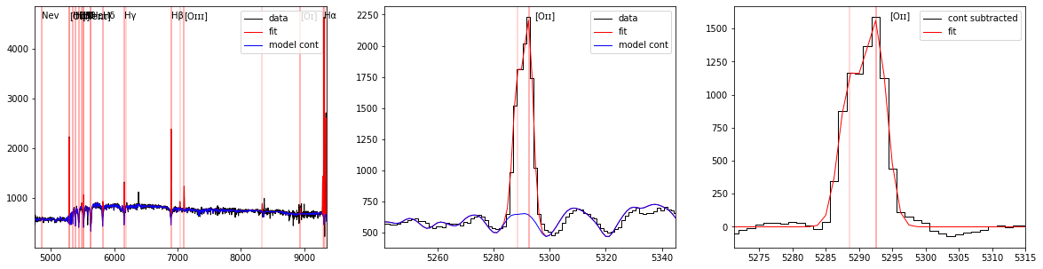
The left panel display the full spectrum (in black) and its continuum fit (in blue) with the location of fitted lines (in red). The central panel display a zoom on the [OII] doublet and the right panel the continuum subtracted spectrum.

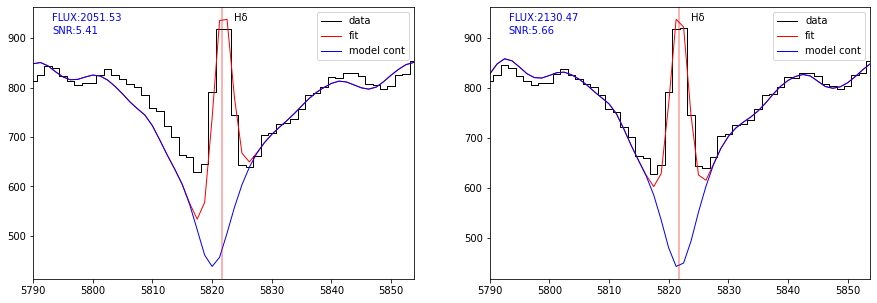
Improving continuum fit¶

From the central panel of the previous plot, one can see that the continuum fit (in blue) is slightly offseted with respect to the data. The reason is that the continuum estimation performed in the first step of the fitting process use a fixed value of z, as given by the input redshift. In that case it is wise to use ziter=True in fit_spec to allow a second iteration.

[8]:

logger = logging.getLogger('pyplatefit')
logger.setLevel('INFO')
res2 = fit_spec(sp, z=0.41892, ziter=True)
logger.setLevel('DEBUG')
fig,ax = plt.subplots(1,2,figsize=(15,5))
plot_fit(ax[0], res, line='HDELTA', margin=30, infoline=['FLUX','SNR'])
plot_fit(ax[1], res2, line='HDELTA', margin=30, infoline=['FLUX','SNR'])

Fitting all lines together¶

In some case, it is better to fit all lines together rather than splitting the fit by families. This is done with the fit_all=True flag.

Note that \({\rm Ly\alpha}\), given its systematic offset with respect to the systemic velocity, is still fitted separatly.

[9]:

logger.setLevel('INFO')
res = fit_spec(sp, z=0.41892, ziter=True, fit_all=True)
logger.setLevel('DEBUG')
res['ztable']

[9]:

Table length=1

FAMILY	VEL	VEL_ERR	Z	Z_ERR	Z_INIT	VDISP	VDISP_ERR	LINE	SNRMAX	SNRSUM	SNRSUM_CLIPPED	NL	NL_CLIPPED	RCHI2	NFEV	STATUS	METHOD
str20	float64	float64	float64	float64	float64	float64	float64	str20	float64	float64	float64	int64	int64	float64	int64	int64	str25
all	3.54	0.71	0.41934	3.38e-06	0.41933	64.55	0.80	HBETA	90.47	75.41	88.28	21	16	14.48	8	3	least_squares

Working with \({\rm Ly\alpha}\)¶

The \({\rm Ly\alpha}\) line is often the only line available at high z. It is generally broad and asymmetric and then it is better fitted with the skewed gaussian model.

[10]:

sp = Spectrum(os.path.join(datadir,'udf10_00723.fits'))
res = fit_spec(sp, z=3.18817)

[DEBUG] Fit continuum
[DEBUG] Fit emission lines
[DEBUG] Preparing data for fit
[DEBUG] Getting lines from default line table...
[DEBUG] 16.7 % of the spectrum is used for fitting.
[DEBUG] Initialize fit
[DEBUG] Init Lya Fit
[DEBUG] added 1 asymetric gaussian to the fit
[DEBUG] Found 1 non resonnant line families to fit
[DEBUG] Init Fit of family forbidden
[DEBUG] Found 14 lines to fit
[DEBUG] added 14 gaussian to the fit
[DEBUG] Found 1 resonnant line families to fit
[DEBUG] Init fitting of family civ1548
[DEBUG] Found 2 lines to fit
[DEBUG] added 2 gaussian to the fit
[DEBUG] Fitting of Line Family: lya
[DEBUG] Lmfit fitting: {'method': 'least_square', 'xtol': 0.001}
[DEBUG] `xtol` termination condition is satisfied. after 11 iterations, reached minimum = 188.100 and redChi2 = 0.308
[DEBUG] Fitting of Line Family: forbidden
[DEBUG] Lmfit fitting: {'method': 'least_square', 'xtol': 0.001}
[DEBUG] Both `ftol` and `xtol` termination conditions are satisfied. after 16 iterations, reached minimum = 209.310 and redChi2 = 0.350
[DEBUG] Fitting of Line Family: civ1548
[DEBUG] Lmfit fitting: {'method': 'least_square', 'xtol': 0.001}
[DEBUG] `xtol` termination condition is satisfied. after 14 iterations, reached minimum = 212.787 and redChi2 = 0.349
[DEBUG] Saving lya results to tablines and ztab
[DEBUG] Saving forbidden results to tablines and ztab
[DEBUG] Saving civ1548 results to tablines and ztab

In the output debug log, one can see that the continuum fit failed. This is the case when the cotniuum is too faint, then a constant is used (median of the continuum).

We also see that in addition to forbidden lines, \({\rm Ly\alpha}\) and the resonnant CIV doublet were fitted separately. However when looking to the ztable, we see that all lines except \({\rm Ly\alpha}\) are below the detection limit.

[11]:

res['ztable']

[11]:

Table length=3

FAMILY	VEL	VEL_ERR	Z	Z_ERR	Z_INIT	VDISP	VDISP_ERR	LINE	SNRMAX	SNRSUM	SNRSUM_CLIPPED	NL	NL_CLIPPED	RCHI2	NFEV	STATUS	METHOD
str20	float64	float64	float64	float64	float64	float64	float64	str20	float64	float64	float64	int64	int64	float64	int64	int64	str25
civ1548	120.59	50.63	3.18985	7.07e-04	3.18817	50.05	68.64	CIV1549b	1.54	1.54	0.00	1	0	0.35	14	3	least_squares
forbidden	-121.11	151.50	3.18648	2.12e-03	3.18817	300.00	124.47	SiIV1403b	1.56	2.08	0.00	8	0	0.35	16	4	least_squares
lyalpha	37.03	21.98	3.18869	3.07e-04	3.18817	263.96	49.61	LYALPHA	7.31	7.31	7.31	1	1	0.31	11	3	least_squares

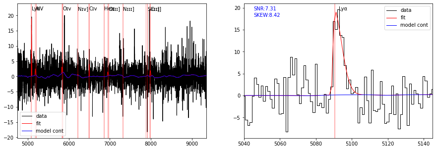
As shown in the following plot, the \({\rm Ly\alpha}\) line is well fitted by a skewed Gaussian with \(\gamma\) positive (SKEW = 8.4), confirming the strong red asymetry of the line profile.

[12]:

fig,ax = plt.subplots(1,2,figsize=(15,5))
plot_fit(ax[0], res)
plot_fit(ax[1], res, line='LYALPHA', infoline=['SNR','SKEW'])

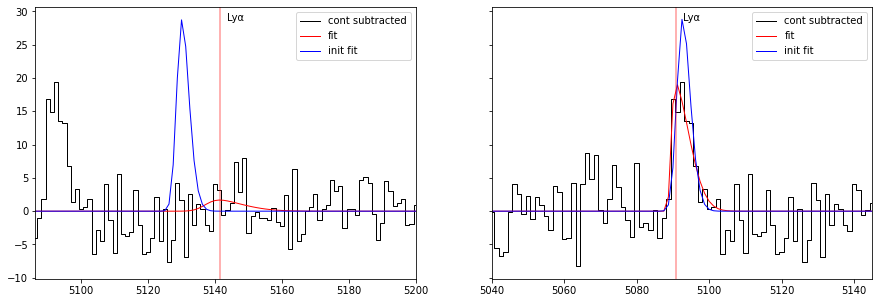
When the initial redshift is poorly known the fit might not converge to the right solution. One can check the provided initial solution with the start=True option in the plot_line. As shown in the left panel of the above plot, the initial solution (in blue) was too far from the left peak to converge to the solution.

In that case it is possible to use the option flag find_lya_vel_offset=True in fit_spec to perform an initail peak search prior to the fit. As it can be seen from the right panel, this help the process to converge to the solution.

However, this option must be used with care as it can easily pick another peaked as initial solution.

[13]:

logger.setLevel('INFO')
res = fit_spec(sp, z=3.22)
res2 = fit_spec(sp, z=3.22, find_lya_vel_offset=True)
fig,ax = plt.subplots(1,2,figsize=(15,5),sharey=True)
plot_fit(ax[0], res, line='LYALPHA', start=True, line_only=True)
plot_fit(ax[1], res2, line='LYALPHA', start=True, line_only=True)

Double peaked \({\rm Ly\alpha}\) line profile¶

In some case, the \({\rm Ly\alpha}\) line profile can display a blue bump or even a double peak. In that case we can use the option flag dble_lyafit=True to perform the double skewed gaussain fit.

[14]:

sp = Spectrum(os.path.join(datadir,'udf10_00106.fits'))
res = fit_spec(sp, z=3.27554, dble_lyafit=True)

[15]:

fig,ax = plt.subplots(1,1,figsize=(7,5),sharey=True)
plot_fit(ax, res, line='LYALPHA1')

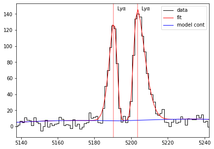
The two line peaks are fitted together with two skewed gaussian. The two profiles are names LYALPHA1 and LYALPHA2 for the blue and red components respectively. The paramaters of the fit are the velocity (or redshift) measured as the center of the peak separation (SEP), the flux, velocity dispersion and skewness of each peak. Note that the redshit given by this fit is the center of the two peaks and not the peak of the line as it is for a single line fit.

[16]:

lines = res['lines'].copy()
lines = lines[~lines['ISBLEND']]
lines[lines['FAMILY']=='lyalpha']['LINE','VEL','Z','SEP','VDISP','FLUX','SKEW']

[16]:

Table length=2

LINE	VEL	Z	SEP	VDISP	FLUX	SKEW
str20	float64	float64	float64	float64	float64	float64
LYALPHA1	34.18	3.27603	515.83	194.33	680.34	-2.78
LYALPHA2	34.18	3.27603	515.83	307.58	1080.47	4.04

Working with doublets and blends¶

Many lines are double (or more) which can be marginally resolved at the instrumental spectral resolution. For these lines, the fit report the parameters of each lines but also for the blend, adding a b at the end of the line name (eg OII3727b). The returned table has a BLEND column flag which allow to filter in/out these lines.

[17]:

sp = Spectrum(os.path.join(datadir,'mosaic_01102.fits'))
res1 = fit_spec(sp, z=0.6198)
lines = res1['lines'].copy()
lines[lines['ISBLEND']]

[17]:

Table length=1

FAMILY	LINE	ISBLEND	LBDA_REST	DNAME	VEL	VEL_ERR	Z	Z_ERR	Z_INIT	VDINST	VDISP	VDISP_ERR	FLUX	FLUX_ERR	SNR	SKEW	SKEW_ERR	LBDA_OBS	PEAK_OBS	LBDA_LEFT	LBDA_RIGHT	FWHM_OBS	NSTD	LBDA_LNSTD	LBDA_RNSTD	BLEND	EQW	EQW_ERR	CONT_OBS	CONT	CONT_ERR
str20	str20	bool	float64	str20	float64	float64	float64	float64	float64	float64	float64	float64	float64	float64	float64	float64	float64	float64	float64	float64	float64	float64	float64	float64	float64	int64	float64	float64	float64	float64	float64
forbidden	OII3727b	True	3728.48	[Oɪɪ]	5.98	11.07	0.61983	5.98e-05	0.61980	0.00	37.40	15.08	165.30	27.75	5.96	0.00	0.00	6037.85	32.01	6034.08	6041.61	3.01	0.00	0.00	0.00	3727	-10.51	2.48	9.71	15.73	12.24

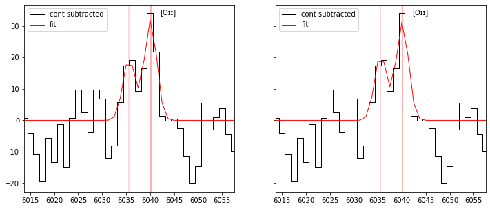
In some case we may also want to constrain the line ratios to avoid unphysical fit. This is activated with the option flag use_line_ratios=True.

By default the following line ratios are defined:

\({\rm \left( 0.3 < \frac{OII_{3729}}{OII_{3726}} < 1.5 \right)}\) and \({\rm \left( 0.6 < \frac{CIII_{1909}}{CIII_{1907}} < 1.2 \right)}\)

We will see later how to define new lines ratio.

[18]:

res2 = fit_spec(sp, z=0.6198, use_line_ratios=True)
for res in [res1,res2]:
    lines = res['lines'].copy()
    r1 = lines[lines['LINE']=='OII3726'][0]
    r2 = lines[lines['LINE']=='OII3729'][0]
    r21 = r2['FLUX']/r1['FLUX']
    print('ratio: ',r21)

ratio:  1.6316695024665604
ratio:  1.4999997928730038

[19]:

fig,ax = plt.subplots(1,2,figsize=(12,5), sharey=True)
plot_fit(ax[0], res1, line='OII3726', line_only=True, margin=20)
plot_fit(ax[1], res2, line='OII3726', line_only=True, margin=20)

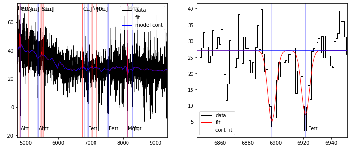
Fitting absorption lines¶

The program offer an option to fit absorption lines. This is activated with the flag fitabs=True. The absorption lines fit is performed in a third step, after the emission line fit. The emission lines are subtracted from the original spectrum, a polynomial is performed to subtract the low order continuum and then all absorption lines are fitted simultaneously similarely to the emission line fit.

Note that, in the case of strong emission lines, the lines residuals left by the emission line fitting, together with the accuracy of the polynomial continuum fit, may lead to inaccurate results in the absorption lines fit.

[20]:

sp = Spectrum(os.path.join(datadir,'DR2_001028.fits'))
res = fit_spec(sp, z=1.90578, fitabs=True)

[21]:

res['ztable']

[21]:

Table length=3

FAMILY	VEL	VEL_ERR	Z	Z_ERR	Z_INIT	VDISP	VDISP_ERR	LINE	SNRMAX	SNRSUM	SNRSUM_CLIPPED	NL	NL_CLIPPED	RCHI2	NFEV	STATUS	METHOD
str20	float64	float64	float64	float64	float64	float64	float64	str20	float64	float64	float64	int64	int64	float64	int64	int64	str25
forbidden	-52.84	34.80	1.90527	3.37e-04	1.90578	88.02	31.01	CII2326b	2.78	4.21	0.00	8	0	1.26	18	3	least_squares
mgii2796	279.76	17.56	1.90849	1.70e-04	1.90578	56.51	21.07	MgII2799b	4.72	4.72	4.72	1	1	1.29	27	3	least_squares
abs	-16.32	5.77	1.90562	5.60e-05	1.90578	116.56	6.00	MgII2799b	16.50	23.97	28.58	10	8	0.74	6	3	least_squares

[22]:

fig,ax = plt.subplots(1,2,figsize=(12,5))
plot_fit(ax[0], res)
plot_fit(ax[1], res, line='FeII2374', abs_line=True)

[23]:

fig,ax = plt.subplots(1,3,figsize=(12,5))
plot_fit(ax[0], res, line='MgII2796', legend=False)
plot_fit(ax[1], res, line='MgII2796', line_only=True, legend=False)
plot_fit(ax[2], res, line='MgII2796', abs_line=True, legend=False)

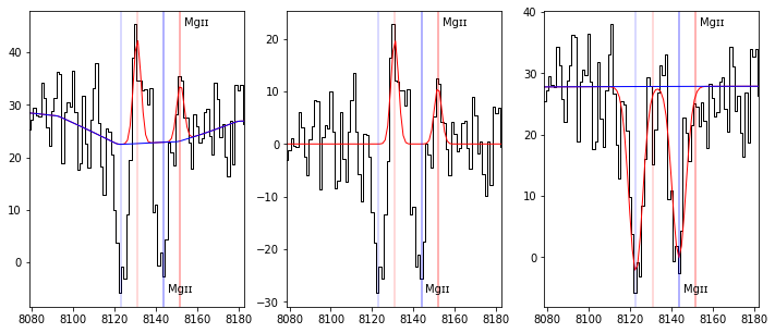
One can see in these last plots that both MgII absorptions and the resonnant MgII emission doublet are raisonably well fitted.

For passive galaxy with no emission line, one can also skip the emission line fitting by setting the fitlines=False flag.

[24]:

res = fit_spec(sp, z=1.90578, fitabs=True, fitlines=False)
res['ztable']

[24]:

Table length=1

FAMILY	VEL	VEL_ERR	Z	Z_ERR	Z_INIT	VDISP	VDISP_ERR	LINE	SNRMAX	SNRSUM	SNRSUM_CLIPPED	NL	NL_CLIPPED	RCHI2	NFEV	STATUS	METHOD
str20	float64	float64	float64	float64	float64	float64	float64	str20	float64	float64	float64	int64	int64	float64	int64	int64	str25
abs	-21.17	5.63	1.90557	5.45e-05	1.90578	108.82	5.93	MgII2799b	15.76	23.26	27.75	10	8	0.79	7	3	least_squares

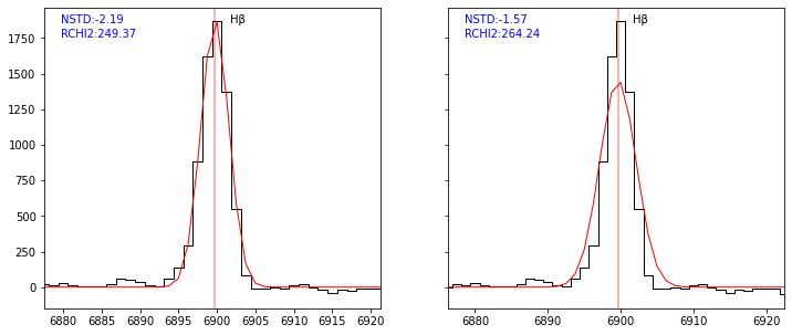
Fitting accuracy¶

To judge the fit accuracy pyplatefit provide two indicators:

The reduced chi square value for the simultaneous fit of all lines for each family. This value is given by the lmfit least square routine.

To assess the goodness of the fit for each individual lines, the parameter NSTD is returned in the lines table. NSTD is the log10 of the standard deviation of the residuals after normalisation of the flux by the total model flux. Computation is performed in a window centered on the line peak with a width relative to the FWHM of the line. The window wavelengths limits are saved in the table as LBDA_LNSTD and LBDA_RNSTD. The smaller NSTD, the better. Typical good line fit have NSTD lower than -2.

[25]:

sp = Spectrum(os.path.join(datadir,'udf10_00002.fits'))
res1 = fit_spec(sp, z=0.41892)
res2 = fit_spec(sp, z=0.41892, linepars=dict(vdisp=(100,150,300)))

[26]:

fig,ax = plt.subplots(1,2,figsize=(12,5), sharey=True)
kw = dict(line='HBETA', line_only=True, margin=20, infoline=['NSTD'], infoz=['RCHI2'], legend=False)
plot_fit(ax[0], res1, **kw)
plot_fit(ax[1], res2, **kw)

Improving error estimate using MCMC¶

Although the lmfit least square routine provide in general a reasonnable estimation of errors, it may give wrong results when the line is very noisy or when model parameters are strongly correlated. This is for example the case for the double \({\rm Ly\alpha}\) line fit.

In that case, pyplatefit has an option to evaluate the errors using Markov Chain Monte Carlo using the emcee python module, through the lmfit interface. These options are set with two boolean flags: mcmc_lya and mcmc_all, to run the MCMC for respectively only the \({\rm Ly\alpha}\) line or all emission and absorption lines.

Please note that this option is quite cpu intensive and thus it is recommended to activate only if this is requested.

We use the previous example to show how it works. We compare the \({\rm Ly\alpha}\) fit with and without the MCMC option.

[27]:

sp = Spectrum(os.path.join(datadir,'udf10_00723.fits'))
res0 = fit_spec(sp, z=3.18817, lines=['LYALPHA'])

[28]:

logger.setLevel('DEBUG')
sp = Spectrum(os.path.join(datadir,'udf10_00723.fits'))
res1 = fit_spec(sp, z=3.18817, lines=['LYALPHA'], mcmc_lya=True)

[DEBUG] Fit continuum
[DEBUG] Fit emission lines
[DEBUG] Preparing data for fit
[DEBUG] Getting lines from default line table...
[DEBUG] 1.9 % of the spectrum is used for fitting.
[DEBUG] Initialize fit
[DEBUG] Init Lya Fit
[DEBUG] added 1 asymetric gaussian to the fit
[DEBUG] Found 0 non resonnant line families to fit
[DEBUG] Found 0 resonnant line families to fit
[DEBUG] Fitting of Line Family: lya
[DEBUG] Lmfit fitting: {'method': 'least_square', 'xtol': 0.001}
[DEBUG] `xtol` termination condition is satisfied. after 11 iterations, reached minimum = 23.191 and redChi2 = 0.346
[DEBUG] Emcee fitting: {'method': 'emcee', 'is_weighted': True, 'steps': 10000, 'nwalkers': 40, 'progress': True, 'run_mcmc_kwargs': {'skip_initial_state_check': False}}

100%|██████████| 10000/10000 [01:04<00:00, 156.03it/s]

[DEBUG] status 1 after 400000 fcn eval, chain size ratio = 1.5 max autocorr time = 130.6 mean acceptance fraction = 0.53, reached minimum = 23.446 and redChi2 = 0.350
[DEBUG] Saving lya results to tablines and ztab

[29]:

fig,ax = plt.subplots(1,2,figsize=(12,5), sharey=True)
kw = dict(line='LYALPHA', line_only=True, margin=20, infoline=['FLUX','SNR'], infoz=['METHOD'], legend=False)
plot_fit(ax[0], res0, **kw)
plot_fit(ax[1], res1, **kw)

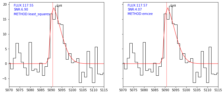
As shown in the plot above the solutions are nearly identical. This is expected given that the MCMC routine use as starting point the least-square solution, and only then explore the parameter space to derive the probability distribution. Note however that the S/N derived is much lower (70%) than the one returned by the least square routine.

To check if the MCMC solution has converged we need to check the autocorrelation time returned by the routine. According to the emcee documentation, the chain length (Steps) must be large enough with respect to the autocorrelation time (Acor). In practice it is recommended to have \(\rm Steps > 50 \times Acor\) for all parameters. The program print the minimum value of 1.5 for the chain ratio which indicate that we are fine.

We can also have a more detailed view of the returned parameters using the print_res function.

[30]:

print_res(res1, 'lyalpha')

[30]:

Table masked=True length=5

Name	Min_bound	Max_bound	Init_value	Value	Median	Init_Std	Std	Acor	Acor_ratio	Min_p99	Min_p95	Max_p95	Max_p99
bytes40	float32	float32	float32	float32	float32	float32	float32	float32	float32	float32	float32	float32	float32
dv_lyalpha	-500.000	500.000	-30.330	-30.328	-24.327	23.283	57.119	130.624	1.531	--	--	--	--
vdisp_lyalpha	50.000	700.000	263.959	263.965	274.027	52.560	92.983	67.510	2.963	--	--	--	--
lyalpha_LYALPHA_asymgauss_l0	-inf	inf	1215.670	1215.670	--	--	nan	--	--	--	--	--	--
lyalpha_LYALPHA_asymgauss_flux	0.000	inf	117.554	117.567	118.993	17.028	28.853	58.172	3.438	--	--	--	--
lyalpha_LYALPHA_asymgauss_asym	-1.000	10.000	8.425	8.434	5.263	6.263	3.323	95.085	2.103	--	--	--	--

The returned table gives detailed information for all model parameters. For each parameter we have the bounds (Min_bound and Max_bound), the initial value and standard deviation (Init_value, Init_Std) which are the one returned by the least-square fit, the maximum likehood value (Value), the median value (Median) of the distribution and the standard deviation (Std). We can also see the autocorrelation time (Acor) and the ratio discussed above (Acor_ratio). If the MCMC has converged we should have Acor_ratio larger than 1 for all parameters. For example the flux error estimate has a very large value of 3.7 and then we can be sure that the errors is well estimated.

We will see later that the parameter Acor_ratio is also returned as par_RTAU in the lines table.

Now we run the fit for all lines for the same spectra, using the mcmc_all flag.

[31]:

sp = Spectrum(os.path.join(datadir,'udf10_00723.fits'))
res2 = fit_spec(sp, z=3.18817, mcmc_all=True)

[DEBUG] Fit continuum
[DEBUG] Fit emission lines
[DEBUG] Preparing data for fit
[DEBUG] Getting lines from default line table...
[DEBUG] 16.7 % of the spectrum is used for fitting.
[DEBUG] Initialize fit
[DEBUG] Init Lya Fit
[DEBUG] added 1 asymetric gaussian to the fit
[DEBUG] Found 1 non resonnant line families to fit
[DEBUG] Init Fit of family forbidden
[DEBUG] Found 14 lines to fit
[DEBUG] added 14 gaussian to the fit
[DEBUG] Found 1 resonnant line families to fit
[DEBUG] Init fitting of family civ1548
[DEBUG] Found 2 lines to fit
[DEBUG] added 2 gaussian to the fit
[DEBUG] Fitting of Line Family: lya
[DEBUG] Lmfit fitting: {'method': 'least_square', 'xtol': 0.001}
[DEBUG] `xtol` termination condition is satisfied. after 11 iterations, reached minimum = 188.100 and redChi2 = 0.308
[DEBUG] Emcee fitting: {'method': 'emcee', 'is_weighted': True, 'steps': 10000, 'nwalkers': 40, 'progress': True, 'run_mcmc_kwargs': {'skip_initial_state_check': False}}

100%|██████████| 10000/10000 [00:59<00:00, 166.86it/s]

[DEBUG] status 1 after 400000 fcn eval, chain size ratio = 1.9 max autocorr time = 106.4 mean acceptance fraction = 0.52, reached minimum = 188.341 and redChi2 = 0.309
[DEBUG] Fitting of Line Family: forbidden
[DEBUG] Lmfit fitting: {'method': 'least_square', 'xtol': 0.001}
[DEBUG] Both `ftol` and `xtol` termination conditions are satisfied. after 16 iterations, reached minimum = 209.310 and redChi2 = 0.350
[DEBUG] Emcee fitting: {'method': 'emcee', 'is_weighted': True, 'steps': 10000, 'nwalkers': 160, 'progress': True, 'run_mcmc_kwargs': {'skip_initial_state_check': False}}

100%|██████████| 10000/10000 [10:02<00:00, 16.59it/s]

The chain is shorter than 50 times the integrated autocorrelation time for 16 parameter(s). Use this estimate with caution and run a longer chain!
N/50 = 200;
tau: [618.68915442 538.40293423 562.54241887 614.39365113 550.02117346
 572.08205515 549.5646877  546.86227608 557.1934568  573.14339719
 553.58374741 580.04399232 534.58610532 540.38357826 583.24799832
 592.4571212 ]
[DEBUG] status 0 after 1600000 fcn eval, chain size ratio = 0.3 max autocorr time = 618.7 mean acceptance fraction = 0.16, reached minimum = 210.695 and redChi2 = 0.352
[DEBUG] Fitting of Line Family: civ1548
[DEBUG] Lmfit fitting: {'method': 'least_square', 'xtol': 0.001}
[DEBUG] `xtol` termination condition is satisfied. after 14 iterations, reached minimum = 212.787 and redChi2 = 0.349
[DEBUG] Emcee fitting: {'method': 'emcee', 'is_weighted': True, 'steps': 10000, 'nwalkers': 40, 'progress': True, 'run_mcmc_kwargs': {'skip_initial_state_check': False}}

100%|██████████| 10000/10000 [01:05<00:00, 152.69it/s]

The chain is shorter than 50 times the integrated autocorrelation time for 1 parameter(s). Use this estimate with caution and run a longer chain!
N/50 = 200;
tau: [109.35791379  97.65140256 642.37228804  88.02403696]
[DEBUG] status 0 after 400000 fcn eval, chain size ratio = 0.3 max autocorr time = 642.4 mean acceptance fraction = 0.43, reached minimum = 214.066 and redChi2 = 0.351
[DEBUG] Saving lya results to tablines and ztab
[DEBUG] Saving forbidden results to tablines and ztab
[DEBUG] Saving civ1548 results to tablines and ztab

One can have a summary of the fit by looking to the ztable

[32]:

res2['ztable']

[32]:

Table length=3

FAMILY	VEL	VEL_ERR	Z	Z_ERR	Z_INIT	VDISP	VDISP_ERR	LINE	SNRMAX	SNRSUM	SNRSUM_CLIPPED	NL	NL_CLIPPED	RCHI2	NFEV	STATUS	METHOD	NSTEPS	RCHAIN	NBAD	RCHAIN_CLIP	NBAD_CLIP
str20	float64	float64	float64	float64	float64	float64	float64	str20	float64	float64	float64	int64	int64	float64	int64	int64	str25	int64	float64	int64	float64	int64
civ1548	120.64	258.79	3.18986	3.62e-03	3.18817	49.99	89.84	CIV1549b	1.03	1.03	0.00	1	0	0.35	400000	0	emcee	10000	0.31	1	0.00	0
forbidden	-121.10	226.72	3.18648	3.17e-03	3.18817	300.00	42.78	CIII1909b	1.32	2.14	0.00	8	0	0.35	1600000	0	emcee	10000	0.32	14	0.00	0
lyalpha	37.03	59.93	3.18869	8.37e-04	3.18817	263.94	93.81	LYALPHA	4.11	4.11	4.11	1	1	0.31	400000	1	emcee	10000	1.88	0	1.88	0

One can see from the status value of 0, that the MCMC did not converge for the civ1548 and forbidden families. Indeed the reported value for the chain length ratio (RCHAIN) is below 1. The NBAD column indicate the number of lines that are below 1. All lines have a SNR below 3 as indicated by the zero value of NL_CLIPPED. Note that the SNR value is probably not very reliable because the MCMC did not converge. The velocity dispersion seems also high. We can check this by looking to the bounds value returned by print_res.

[33]:

print_res(res2, 'forbidden')[0:3]

[33]:

Table masked=True length=3

Name	Min_bound	Max_bound	Init_value	Value	Median	Init_Std	Std	Acor	Acor_ratio	Min_p99	Min_p95	Max_p95	Max_p99
bytes40	float32	float32	float32	float32	float32	float32	float32	float32	float32	float32	float32	float32	float32
dv_forbidden	-500.000	500.000	-121.113	-121.104	-74.678	151.501	226.719	618.689	0.323	--	--	--	--
vdisp_forbidden	5.000	300.000	300.000	300.000	268.465	124.474	42.780	538.403	0.371	--	--	--	--
forbidden_NV1238_gauss_l0	-inf	inf	1238.820	1238.820	--	--	nan	--	--	--	--	--	--

As shown above, the least-square fit reach the velocity dispersion bounds. Let’s run the fit separately to see if we obtain a better solution.

[34]:

sp = Spectrum(os.path.join(datadir,'udf10_00723.fits'))
res4 = fit_spec(sp, z=3.18817, mcmc_all=True, lines=['CIII1907','CIII1909'])

[DEBUG] Fit continuum
[DEBUG] Fit emission lines
[DEBUG] Preparing data for fit
[DEBUG] Getting lines from default line table...
[DEBUG] 1.8 % of the spectrum is used for fitting.
[DEBUG] Initialize fit
[DEBUG] Found 1 non resonnant line families to fit
[DEBUG] Init Fit of family forbidden
[DEBUG] Found 2 lines to fit
[DEBUG] added 2 gaussian to the fit
[DEBUG] Found 0 resonnant line families to fit
[DEBUG] Fitting of Line Family: forbidden
[DEBUG] Lmfit fitting: {'method': 'least_square', 'xtol': 0.001}
[DEBUG] `xtol` termination condition is satisfied. after 9 iterations, reached minimum = 19.882 and redChi2 = 0.316
[DEBUG] Emcee fitting: {'method': 'emcee', 'is_weighted': True, 'steps': 10000, 'nwalkers': 40, 'progress': True, 'run_mcmc_kwargs': {'skip_initial_state_check': False}}

100%|██████████| 10000/10000 [01:04<00:00, 155.78it/s]

[DEBUG] status 1 after 400000 fcn eval, chain size ratio = 2.3 max autocorr time = 87.7 mean acceptance fraction = 0.45, reached minimum = 20.591 and redChi2 = 0.327
[DEBUG] Saving forbidden results to tablines and ztab

[35]:

res4['ztable']

[35]:

Table length=1

FAMILY	VEL	VEL_ERR	Z	Z_ERR	Z_INIT	VDISP	VDISP_ERR	LINE	SNRMAX	SNRSUM	SNRSUM_CLIPPED	NL	NL_CLIPPED	RCHI2	NFEV	STATUS	METHOD	NSTEPS	RCHAIN	NBAD	RCHAIN_CLIP	NBAD_CLIP
str20	float64	float64	float64	float64	float64	float64	float64	str20	float64	float64	float64	int64	int64	float64	int64	int64	str25	int64	float64	int64	float64	int64
forbidden	-145.83	276.13	3.18613	3.86e-03	3.18817	82.56	81.25	CIII1909b	1.89	1.89	0.00	1	0	0.33	400000	1	emcee	10000	2.28	0	0.00	0

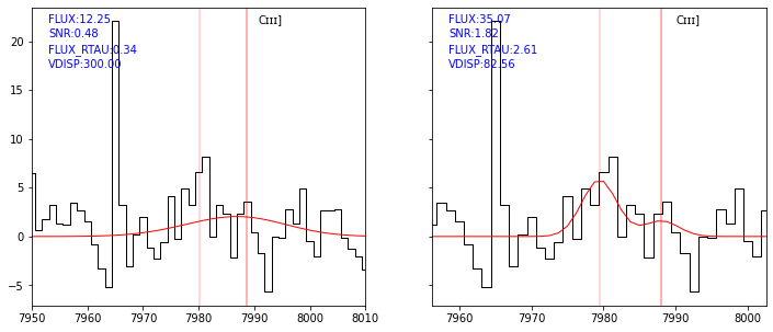
This time the velocity dispersion is ok and the RCHAIN value is ok. This is better shown in the following plot.

[36]:

ltab = res4['lines']
ltab = ltab[(ltab['LINE']=='CIII1907') | (ltab['LINE']=='CIII1909')]
ltab['LINE','SNR','FLUX','FLUX_RTAU','VDISP']

[36]:

Table length=2

LINE	SNR	FLUX	FLUX_RTAU	VDISP
str20	float64	float64	float64	float64
CIII1907	1.82	35.07	2.61	82.56
CIII1909	0.53	9.68	2.35	82.56

[37]:

fig,ax = plt.subplots(1,2,figsize=(12,5), sharey=True)
kw = dict(line='CIII1907', line_only=True, margin=20, infoline=['FLUX','SNR','FLUX_RTAU','VDISP'], legend=False)
plot_fit(ax[0], res2, **kw)
plot_fit(ax[1], res4, **kw)

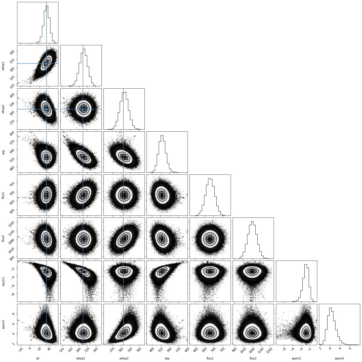
When using the mcmc option, we have access to the full probability distribution of each parameters. The save_proba option will save the 95% and 99% bounds for each parameters. We illustrate this on the double peaked lya fit.

[38]:

sp = Spectrum(os.path.join(datadir,'udf10_00106.fits'))
res = fit_spec(sp, z=3.27554, dble_lyafit=True, lines=['LYALPHA'], mcmc_lya=True, mcmcpars=dict(save_proba=True))

[DEBUG] Fit continuum
[DEBUG] Fit emission lines
[DEBUG] Preparing data for fit
[DEBUG] Getting lines from default line table...
[DEBUG] 2.0 % of the spectrum is used for fitting.
[DEBUG] Initialize fit
[DEBUG] Init Lya Fit
[DEBUG] Using double asymetric gaussian model
[DEBUG] added 1 double asymetric gaussian to the fit
[DEBUG] Found 0 non resonnant line families to fit
[DEBUG] Found 0 resonnant line families to fit
[DEBUG] Fitting of Line Family: lya
[DEBUG] Lmfit fitting: {'method': 'least_square', 'xtol': 0.001}
[DEBUG] `xtol` termination condition is satisfied. after 6 iterations, reached minimum = 46.432 and redChi2 = 0.714
[DEBUG] Emcee fitting: {'method': 'emcee', 'is_weighted': True, 'nwalkers': 80, 'steps': 15000}

100%|██████████| 15000/15000 [04:29<00:00, 55.66it/s]

[DEBUG] status 1 after 1200000 fcn eval, chain size ratio = 2.7 max autocorr time = 110.6 mean acceptance fraction = 0.45, reached minimum = 46.526 and redChi2 = 0.716
[DEBUG] Saving lya results to tablines and ztab

[39]:

print_res(res, 'lyalpha')

[39]:

Table masked=True length=9

Name	Min_bound	Max_bound	Init_value	Value	Median	Init_Std	Std	Acor	Acor_ratio	Min_p99	Min_p95	Max_p95	Max_p99
bytes40	float32	float32	float32	float32	float32	float32	float32	float32	float32	float32	float32	float32	float32
dv_lyalpha	-500.000	500.000	34.180	34.178	34.224	4.830	5.982	97.409	3.080	18.334	23.753	43.785	47.688
vdisp1_lyalpha	50.000	700.000	194.328	194.329	196.491	11.931	14.195	96.791	3.099	160.546	172.276	219.412	228.622
vdisp2_lyalpha	50.000	700.000	307.577	307.555	309.836	11.401	14.025	93.444	3.210	276.797	286.658	333.031	342.889
lyalpha_LYALPHA_dbleasymgauss_l0	-inf	inf	1215.670	1215.670	--	--	nan	--	--	--	--	--	--
lyalpha_LYALPHA_dbleasymgauss_sep	80.000	1000.000	515.832	515.810	514.371	9.661	12.059	97.582	3.074	488.237	495.522	535.751	546.654
lyalpha_LYALPHA_dbleasymgauss_flux1	0.000	inf	680.343	680.268	680.273	21.032	24.558	83.410	3.597	623.565	640.039	720.819	737.965
lyalpha_LYALPHA_dbleasymgauss_flux2	0.000	inf	1080.472	1080.487	1080.355	26.045	30.459	90.018	3.333	1010.326	1030.831	1131.426	1153.226
lyalpha_LYALPHA_dbleasymgauss_asym1	-10.000	0.000	-2.776	-2.777	-2.886	0.497	0.667	110.596	2.713	-5.148	-4.230	-1.939	-1.567
lyalpha_LYALPHA_dbleasymgauss_asym2	0.000	10.000	4.040	4.041	4.219	0.584	0.814	98.229	3.054	2.731	3.103	5.877	6.858

More information is available (see here). For example we can visualize the posterior distributions for the parameters using the corner package:

[40]:

import corner
lmres = res['dline']['lmfit_lya']
names = [e.split('_')[0] for e in lmres.var_names[0:3]] + [e.split('_')[-1] for e in lmres.var_names[3:]]
emcee_plot = corner.corner(lmres.flatchain, labels=names,
                           truths=list(lmres.params.valuesdict().values()))

Selecting and updating emission/absorption lines¶

The program comes with a default line list and provide options to select, adapt and update the line list.

The default line astropy table can be returned by the get_lines function.

[41]:

from pyplatefit import get_lines
get_lines(orig=True)

[41]:

Table length=75

LINE	FAMILY	LBDA_REST	DOUBLET	MAIN	EMI	ABS	RESONANT	DNAME
bytes9	bytes9	float32	int64	bool	bool	bool	bool	bytes10
OVI1032	forbidden	1031.91	1033	False	True	False	False	None
OVI1038	forbidden	1037.61	1033	False	True	False	False	Ovɪ
LYALPHA	balmer	1215.67	0	True	True	False	True	Lyα
NV1238	forbidden	1238.82	1240	False	True	False	False	None
NV1242	forbidden	1242.8	1240	False	True	False	False	NV
SiII1260	ism	1260.42	0	False	False	True	False	Siɪɪ
OI1302	ism	1302.17	1303	False	False	True	False	Oɪ
SiII1304	ism	1304.37	1303	False	False	True	False	Siɪɪ
CII1334	ism	1334.53	0	False	False	True	False	Cɪɪ
SiIV1394	forbidden	1393.76	1403	False	True	True	False	None
...	...	...	...	...	...	...	...	...
MgB	ism	5175.44	0	False	False	True	False	Mgb
HeI5876	forbidden	5877.25	0	False	True	False	False	None
NaD	ism	5891.94	0	False	False	True	False	NaD
OI6300	forbidden	6302.05	0	False	True	False	False	[Oɪ]
NII6548	forbidden	6549.85	0	False	True	False	False	None
HALPHA	balmer	6564.61	0	True	True	True	False	Hα
NII6584	forbidden	6585.28	0	True	True	False	False	None
SII6717	forbidden	6718.29	0	True	True	False	False	None
SII6731	forbidden	6732.67	0	True	True	False	False	[Sɪɪ]
ARIII7135	forbidden	7137.8	0	False	True	False	False	[Arɪɪɪ]

These table contains the following columns:

LINE: the line name. There are no official naming convention for the line but we try to pick up the most commo names currently used.
FAMILY: the family name, currently we have balmer, forbidden and ism.
LBDA_REST: the vacuum wavelength rest frame
DOUBLET: an integer which indicate if non zero, that the line is part of a multiplet. All lines with identical values are belonging to the same multiplet.
MAIN: a boolean flag, indicate if the line is considered as a main line.
EMI: a boolean flag for emission line.
ABS: a boolean flag for absorption lines.
RESONNANT: a boolean flag for resonnant lines.
DNAME: display name used for plots.

When performing the fit it is possible to restrict the fit to some lines.

The option flag major_lines=True wil only fit the main lines.

[42]:

sp = Spectrum(os.path.join(datadir,'udf10_00723.fits'))
res = fit_spec(sp, z=3.18817, major_lines=True)

[DEBUG] Fit continuum
[DEBUG] Fit emission lines
[DEBUG] Preparing data for fit
[DEBUG] Getting lines from default line table...
[DEBUG] 5.3 % of the spectrum is used for fitting.
[DEBUG] Initialize fit
[DEBUG] Init Lya Fit
[DEBUG] added 1 asymetric gaussian to the fit
[DEBUG] Found 1 non resonnant line families to fit
[DEBUG] Init Fit of family forbidden
[DEBUG] Found 2 lines to fit
[DEBUG] added 2 gaussian to the fit
[DEBUG] Found 1 resonnant line families to fit
[DEBUG] Init fitting of family civ1548
[DEBUG] Found 2 lines to fit
[DEBUG] added 2 gaussian to the fit
[DEBUG] Fitting of Line Family: lya
[DEBUG] Lmfit fitting: {'method': 'least_square', 'xtol': 0.001}
[DEBUG] `xtol` termination condition is satisfied. after 11 iterations, reached minimum = 65.515 and redChi2 = 0.343
[DEBUG] Fitting of Line Family: forbidden
[DEBUG] Lmfit fitting: {'method': 'least_square', 'xtol': 0.001}
[DEBUG] `xtol` termination condition is satisfied. after 9 iterations, reached minimum = 88.991 and redChi2 = 0.466
[DEBUG] Fitting of Line Family: civ1548
[DEBUG] Lmfit fitting: {'method': 'least_square', 'xtol': 0.001}
[DEBUG] `xtol` termination condition is satisfied. after 14 iterations, reached minimum = 90.202 and redChi2 = 0.472
[DEBUG] Saving lya results to tablines and ztab
[DEBUG] Saving forbidden results to tablines and ztab
[DEBUG] Saving civ1548 results to tablines and ztab

[43]:

res['lines']

[43]:

Table length=7

FAMILY	LINE	ISBLEND	LBDA_REST	DNAME	VEL	VEL_ERR	Z	Z_ERR	Z_INIT	VDINST	VDISP	VDISP_ERR	FLUX	FLUX_ERR	SNR	SKEW	SKEW_ERR	LBDA_OBS	PEAK_OBS	LBDA_LEFT	LBDA_RIGHT	FWHM_OBS	NSTD	LBDA_LNSTD	LBDA_RNSTD	BLEND	EQW	EQW_ERR	CONT_OBS	CONT	CONT_ERR
str20	str20	bool	float64	str20	float64	float64	float64	float64	float64	float64	float64	float64	float64	float64	float64	float64	float64	float64	float64	float64	float64	float64	float64	float64	float64	int64	float64	float64	float64	float64	float64
lyalpha	LYALPHA	False	1215.67	Lyα	37.03	23.18	3.18869	3.24e-04	3.18817	65.68	263.96	52.32	117.55	16.95	6.94	8.42	6.23	5090.64	19.33	5089.47	5095.13	5.66	-1.57	5087.12	5104.10	0	--	--	-0.02	-0.08	14.53
civ1548	CIV1548	False	1548.20	None	120.59	58.91	3.18985	8.23e-04	3.18817	46.46	50.05	79.86	0.00	7.19	0.00	0.00	0.00	6484.94	0.00	6483.20	6486.68	3.48	-0.90	6479.72	6500.92	1549	--	--	-0.09	-0.38	11.46
civ1548	CIV1549b	True	1549.48	Cɪᴠ	120.59	58.91	3.18985	8.23e-04	3.18817	0.00	50.05	79.86	15.61	11.77	1.33	0.00	0.00	6490.32	4.21	6483.20	6497.44	3.48	0.00	0.00	0.00	1549	--	--	-0.11	-0.48	11.38
civ1548	CIV1550	False	1550.77	Cɪᴠ	120.59	58.91	3.18985	8.23e-04	3.18817	46.36	50.05	79.86	15.61	11.77	1.33	0.00	0.00	6495.70	4.21	6493.96	6497.44	3.48	-0.90	6479.72	6500.92	1549	--	--	-0.12	-0.50	11.37
forbidden	CIII1907	False	1906.68	None	-145.80	44.00	3.18613	6.15e-04	3.18817	36.73	82.54	38.21	35.07	16.11	2.18	0.00	0.00	7979.42	5.82	7976.59	7982.25	5.66	-1.17	7970.92	7996.50	1909	--	--	-0.08	-0.32	13.28
forbidden	CIII1909b	True	1907.71	Cɪɪɪ]	-145.80	44.00	3.18613	6.15e-04	3.18817	0.00	82.54	38.21	44.75	18.52	2.42	0.00	0.00	7983.71	5.82	7976.59	7990.83	5.67	0.00	0.00	0.00	1909	--	--	-0.08	-0.35	13.26
forbidden	CIII1909	False	1908.73	Cɪɪɪ]	-145.80	44.00	3.18613	6.15e-04	3.18817	36.70	82.54	38.21	9.68	9.22	1.05	0.00	0.00	7988.00	1.60	7985.16	7990.83	5.67	-1.17	7970.92	7996.50	1909	--	--	-0.08	-0.33	13.29

It is also possible to fit only a subset of lines by providing the list of lines to fit

[44]:

res = fit_spec(sp, z=3.18817, lines=['LYALPHA','CIII1907','CIII1909'])
res['lines']

[DEBUG] Fit continuum
[DEBUG] Fit emission lines
[DEBUG] Preparing data for fit
[DEBUG] Getting lines from default line table...
[DEBUG] 3.7 % of the spectrum is used for fitting.
[DEBUG] Initialize fit
[DEBUG] Init Lya Fit
[DEBUG] added 1 asymetric gaussian to the fit
[DEBUG] Found 1 non resonnant line families to fit
[DEBUG] Init Fit of family forbidden
[DEBUG] Found 2 lines to fit
[DEBUG] added 2 gaussian to the fit
[DEBUG] Found 0 resonnant line families to fit
[DEBUG] Fitting of Line Family: lya
[DEBUG] Lmfit fitting: {'method': 'least_square', 'xtol': 0.001}
[DEBUG] `xtol` termination condition is satisfied. after 11 iterations, reached minimum = 46.069 and redChi2 = 0.344
[DEBUG] Fitting of Line Family: forbidden
[DEBUG] Lmfit fitting: {'method': 'least_square', 'xtol': 0.001}
[DEBUG] `xtol` termination condition is satisfied. after 9 iterations, reached minimum = 69.546 and redChi2 = 0.519
[DEBUG] Saving lya results to tablines and ztab
[DEBUG] Saving forbidden results to tablines and ztab

[44]:

Table length=4

FAMILY	LINE	ISBLEND	LBDA_REST	DNAME	VEL	VEL_ERR	Z	Z_ERR	Z_INIT	VDINST	VDISP	VDISP_ERR	FLUX	FLUX_ERR	SNR	SKEW	SKEW_ERR	LBDA_OBS	PEAK_OBS	LBDA_LEFT	LBDA_RIGHT	FWHM_OBS	NSTD	LBDA_LNSTD	LBDA_RNSTD	BLEND	EQW	EQW_ERR	CONT_OBS	CONT	CONT_ERR
str20	str20	bool	float64	str20	float64	float64	float64	float64	float64	float64	float64	float64	float64	float64	float64	float64	float64	float64	float64	float64	float64	float64	float64	float64	float64	int64	float64	float64	float64	float64	float64
lyalpha	LYALPHA	False	1215.67	Lyα	37.03	23.20	3.18869	3.24e-04	3.18817	65.68	263.96	52.38	117.55	16.97	6.93	8.42	6.24	5090.64	19.33	5089.47	5095.13	5.66	-1.57	5087.12	5104.10	0	--	--	-0.02	-0.08	14.53
forbidden	CIII1907	False	1906.68	None	-145.80	46.43	3.18613	6.49e-04	3.18817	36.73	82.54	40.33	35.07	17.00	2.06	0.00	0.00	7979.42	5.82	7976.59	7982.25	5.66	-1.17	7970.92	7996.50	1909	--	--	-0.08	-0.32	13.28
forbidden	CIII1909b	True	1907.71	Cɪɪɪ]	-145.80	46.43	3.18613	6.49e-04	3.18817	0.00	82.54	40.33	44.75	19.54	2.29	0.00	0.00	7983.71	5.82	7976.59	7990.83	5.67	0.00	0.00	0.00	1909	--	--	-0.08	-0.35	13.26
forbidden	CIII1909	False	1908.73	Cɪɪɪ]	-145.80	46.43	3.18613	6.49e-04	3.18817	36.70	82.54	40.33	9.68	9.73	0.99	0.00	0.00	7988.00	1.60	7985.16	7990.83	5.67	-1.17	7970.92	7996.50	1909	--	--	-0.08	-0.33	13.29

Finally, it is also possible to provide its own table. It must have the same format than the default table.

In the following example, we retreive the default lines table and set the RESONNANT flag to False for the CIV1548,1550 lines. We then run fit_spec and provide the modified lines table. Now the CIV doublet is fitted together with the other forbidden lines.

[45]:

mylines = get_lines(orig=True)
mylines['RESONANT'][(mylines['LINE']=='CIV1548') | (mylines['LINE']=='CIV1550')] = False
res = fit_spec(sp, z=3.18817, lines=mylines, major_lines=True)
res['ztable']

[DEBUG] Fit continuum
[DEBUG] Fit emission lines
[DEBUG] Preparing data for fit
[DEBUG] Getting lines from user line table...
[DEBUG] 5.3 % of the spectrum is used for fitting.
[DEBUG] Initialize fit
[DEBUG] Init Lya Fit
[DEBUG] added 1 asymetric gaussian to the fit
[DEBUG] Found 1 non resonnant line families to fit
[DEBUG] Init Fit of family forbidden
[DEBUG] Found 4 lines to fit
[DEBUG] added 4 gaussian to the fit
[DEBUG] Found 0 resonnant line families to fit
[DEBUG] Fitting of Line Family: lya
[DEBUG] Lmfit fitting: {'method': 'least_square', 'xtol': 0.001}
[DEBUG] `xtol` termination condition is satisfied. after 11 iterations, reached minimum = 65.515 and redChi2 = 0.343
[DEBUG] Fitting of Line Family: forbidden
[DEBUG] Lmfit fitting: {'method': 'least_square', 'xtol': 0.001}
[DEBUG] `xtol` termination condition is satisfied. after 22 iterations, reached minimum = 88.646 and redChi2 = 0.469
[DEBUG] Saving lya results to tablines and ztab
[DEBUG] Saving forbidden results to tablines and ztab

[45]:

Table length=2

FAMILY	VEL	VEL_ERR	Z	Z_ERR	Z_INIT	VDISP	VDISP_ERR	LINE	SNRMAX	SNRSUM	SNRSUM_CLIPPED	NL	NL_CLIPPED	RCHI2	NFEV	STATUS	METHOD
str20	float64	float64	float64	float64	float64	float64	float64	str20	float64	float64	float64	int64	int64	float64	int64	int64	str25
forbidden	121.00	155.52	3.18986	2.17e-03	3.18817	172.35	133.22	CIV1549b	1.35	1.79	0.00	2	0	0.47	22	3	least_squares
lyalpha	37.03	23.18	3.18869	3.24e-04	3.18817	263.96	52.32	LYALPHA	6.94	6.94	6.94	1	1	0.34	11	3	least_squares

Adjusting fit parameters¶

A number of parameters can be changed to adapt the fitting parameters, update bounds, add new line ratios, etc. These parameters are given to fit_spec as python dictionary.

The linepars dictionary is used to define bounds and line ratios of the fitted variable. It can have the following items: - vel = (vmin,vinit,vmax): bounds and initial values of the velocity with respect to the given redshift. Default is (-500,0,500) km/s. Used for all line families except absorption lines.

vdisp = (vmin,vinit,vmax): bounds and initial values of the rest-frame velocity dispersion. Default is (5,50,300) km/s. Used for all line families except \({\rm Ly\alpha}\) and absorption lines.
velabs = (vmin,vinit,vmax): bounds and initial values of the velocity with respect to the given redshift. Default is (-500,0,500) km/s. Used for absorption lines.
vdispabs = (vmin,vinit,vmax): bounds and initial values of the rest-frame velocity dispersion. Default is (5,50,300) km/s. Used for absorption lines.
vdisp_lya = (vmin,vinit,vmax): bounds and initial values of the rest-frame \({\rm Ly\alpha}\) velocity dispersion. Default is (50,150,700) km/s.
gamma_lya = (vmin,vinit,vmax): bounds and initial values of the skewed \({\rm \gamma \, Ly\alpha}\) parameter. Default is (-1,0,10).
sep_2lya = (vmin,vinit,vmax): bounds and initial values of the peak separation for double \({\rm Ly\alpha}\) fit. Default is (80,500,1000) km/s.
gamma_2lya1 = (vmin,vinit,vmax): bounds and initial values of the skewed \({\rm \gamma \, Ly\alpha}\) parameter for the blue line. Default is (-10,-2,0).
gamma_2lya2 = (vmin,vinit,vmax): bounds and initial values of the skewed \({\rm \gamma \, Ly\alpha}\) parameter for the red line. Default is (0,2,10).
line_ratios = list of lines ratio bounds. default is [(“CIII1907”, “CIII1909”, 0.6, 1.2),(“OII3726”, “OII3729”, 0.3, 1.5)]
polydegabs = polynomial degree for continuum fit prior to absorption fit, default 12
polyiterabs = maximum of sig-clip iteration for continuum fit prior to absorption fit, default 3
polywmask = window half size used form masking in polynomial fit prior to absorption fit, default 3.0 Angstroem
windmax = window half size to find peak to estimate initial value for the fitting process (default 10 Angstroem)
minsnr = minimum SNR value used to clip for ztable computation, default 3.0
nstd_relsize = relative size with respect to FWHM for line NSTD estimate, default 3.0

Additional parameters for the MCMC error estimate are given in the mcmpars dictionary: - steps = length of the MCMC chain. Default is 0, which translate to 10000, except for double \(/rm Ly\alpha\) fit where it is 15000. If the process has not converged this is the parameter to adjust. - progress = display a running bar (True/False), default True - nworkers = number of workers. Dafult is 0, which translate to ten times the number of fitted parameters - save_proba = if True, save the 1%, 5%, 95% and 99% percentile for all variables.

For example to constrain the velocity dispersion and the emission line ratio between MgII2796,2803 you have to run the following.

[46]:

sp = Spectrum(os.path.join(datadir,'DR2_001028.fits'))
ratio = [("MgII2796", "MgII2803", 0.5, 1.5)]
params = dict(line_ratios=ratio, vdisp=(5,10,50))
res = fit_spec(sp, z=1.90578, linepars=params)

[DEBUG] Fit continuum
[DEBUG] Fit emission lines
[DEBUG] Preparing data for fit
[DEBUG] Getting lines from default line table...
[DEBUG] 12.7 % of the spectrum is used for fitting.
[DEBUG] Initialize fit
[DEBUG] Found 1 non resonnant line families to fit
[DEBUG] Init Fit of family forbidden
[DEBUG] Found 15 lines to fit
[DEBUG] added 15 gaussian to the fit
[DEBUG] Found 1 resonnant line families to fit
[DEBUG] Init fitting of family mgii2796
[DEBUG] Found 2 lines to fit
[DEBUG] added 2 gaussian to the fit
[DEBUG] Fitting of Line Family: forbidden
[DEBUG] Lmfit fitting: {'method': 'least_square', 'xtol': 0.001}
[DEBUG] `xtol` termination condition is satisfied. after 17 iterations, reached minimum = 569.896 and redChi2 = 1.264
[DEBUG] Fitting of Line Family: mgii2796
[DEBUG] Lmfit fitting: {'method': 'least_square', 'xtol': 0.001}
[DEBUG] `xtol` termination condition is satisfied. after 13 iterations, reached minimum = 599.141 and redChi2 = 1.291
[DEBUG] Saving forbidden results to tablines and ztab
[DEBUG] Saving mgii2796 results to tablines and ztab

[47]:

res['ztable']

[47]:

Table length=2

FAMILY	VEL	VEL_ERR	Z	Z_ERR	Z_INIT	VDISP	VDISP_ERR	LINE	SNRMAX	SNRSUM	SNRSUM_CLIPPED	NL	NL_CLIPPED	RCHI2	NFEV	STATUS	METHOD
str20	float64	float64	float64	float64	float64	float64	float64	str20	float64	float64	float64	int64	int64	float64	int64	int64	str25
forbidden	-64.30	20.15	1.90516	1.95e-04	1.90578	50.00	22.80	CII2326b	4.62	4.62	4.62	8	1	1.26	17	3	least_squares
mgii2796	274.95	16.10	1.90845	1.56e-04	1.90578	50.00	20.03	MgII2799b	4.74	4.74	4.74	1	1	1.29	13	3	least_squares

The minpars dictionary is used for the minimization process with lmfit. The default items are: - method = ‘least_squares’, name of the lmfit minimization method - xtol = 0.001, tolerance requested on fitted parameters

The name of parameters are function of the selected minimization, see lmfit minimization and scipy minimization for the list of minimization and associated parameters.

For example, to add a tolerance on the residual and a maxmim number number of function evaluation, given scipy least_squares documentation we will use the following:

[48]:

params = dict(method='least_squares', xtol=1.e-3, ftol=1.e-3, max_nfev=200)
logger.setLevel('DEBUG')
res = fit_spec(sp, z=1.90578, minpars=params)
logger.setLevel('INFO')

[DEBUG] Fit continuum
[DEBUG] Fit emission lines
[DEBUG] Preparing data for fit
[DEBUG] Getting lines from default line table...
[DEBUG] 12.7 % of the spectrum is used for fitting.
[DEBUG] Initialize fit
[DEBUG] Found 1 non resonnant line families to fit
[DEBUG] Init Fit of family forbidden
[DEBUG] Found 15 lines to fit
[DEBUG] added 15 gaussian to the fit
[DEBUG] Found 1 resonnant line families to fit
[DEBUG] Init fitting of family mgii2796
[DEBUG] Found 2 lines to fit
[DEBUG] added 2 gaussian to the fit
[DEBUG] Fitting of Line Family: forbidden
[DEBUG] Lmfit fitting: {'method': 'least_squares', 'xtol': 0.001, 'ftol': 0.001, 'max_nfev': 200}
[DEBUG] `ftol` termination condition is satisfied. after 6 iterations, reached minimum = 567.640 and redChi2 = 1.259
[DEBUG] Fitting of Line Family: mgii2796
[DEBUG] Lmfit fitting: {'method': 'least_squares', 'xtol': 0.001, 'ftol': 0.001, 'max_nfev': 200}
[DEBUG] `ftol` termination condition is satisfied. after 23 iterations, reached minimum = 599.069 and redChi2 = 1.291
[DEBUG] Saving forbidden results to tablines and ztab
[DEBUG] Saving mgii2796 results to tablines and ztab

We can also use try a different minimization routine. For example, the Nelder-Mead simplex algorithm. But note that it use a much larger number of iterations.

[49]:

params = dict(method='nelder', options=dict(xtol=1.e-3))
logger.setLevel('DEBUG')
res = fit_spec(sp, z=1.90578, minpars=params)
logger.setLevel('INFO')

[DEBUG] Fit continuum
[DEBUG] Fit emission lines
[DEBUG] Preparing data for fit
[DEBUG] Getting lines from default line table...
[DEBUG] 12.7 % of the spectrum is used for fitting.
[DEBUG] Initialize fit
[DEBUG] Found 1 non resonnant line families to fit
[DEBUG] Init Fit of family forbidden
[DEBUG] Found 15 lines to fit
[DEBUG] added 15 gaussian to the fit
[DEBUG] Found 1 resonnant line families to fit
[DEBUG] Init fitting of family mgii2796
[DEBUG] Found 2 lines to fit
[DEBUG] added 2 gaussian to the fit
[DEBUG] Fitting of Line Family: forbidden
[DEBUG] Lmfit fitting: {'method': 'nelder', 'options': {'xtol': 0.001}}
[DEBUG] Maximum number of function evaluations has been exceeded. after 3401 iterations, reached minimum = 571.309 and redChi2 = 1.267
[DEBUG] Fitting of Line Family: mgii2796
[DEBUG] Lmfit fitting: {'method': 'nelder', 'options': {'xtol': 0.001}}
[DEBUG] Optimization terminated successfully. after 172 iterations, reached minimum = 637.016 and redChi2 = 1.373
[DEBUG] Saving forbidden results to tablines and ztab
[DEBUG] Saving mgii2796 results to tablines and ztab

LSF¶

By default, the reported rest frame velocity dispersion are corrected from the instrumental LSF. It is possible to disable this correction by settings lsf=None in fit_spec.

The LSF model is the following MUSE LSF model: \({\rm FWHM \left(\lambda\right) = 5.19939 - 7.56746 \, 10^{-04} \lambda + 4.93397 \, 10^{-08} \lambda^2}\) with FWHM in Angstroem.

It is possible to use its own LSF model by giving his own function \({\rm FWHM \left(\lambda\right)}\), like in the following:

[50]:

import numpy as np
def mylsf(lbda):
    return np.interp(lbda, [4750,9300], [3.5,3.2])

logger.setLevel('INFO')
sp = Spectrum(os.path.join(datadir, 'udf10_00002.fits'))
res0 = fit_spec(sp, z=0.41892)
res1 = fit_spec(sp, z=0.41892, lsf=mylsf)
res2 = fit_spec(sp, z=0.41892, lsf=None)
for res in [res0,res1,res2]:
    lines = res['lines']
    r = lines[lines['LINE']=='OIII5007'][0]
    vdinst = r['VDINST'] if 'VDINST' in lines.columns else 0
    print(f"VDINST={vdinst:.2f} VDISP={r['VDISP']:.2f} FWHM_OBS={r['FWHM_OBS']:.2f}")

VDINST=41.44 VDISP=66.65 FWHM_OBS=4.38
VDINST=59.91 VDISP=54.75 FWHM_OBS=4.53
VDINST=0.00 VDISP=84.04 FWHM_OBS=4.69

Advanced usage¶

To perform specific operation, one could use the Pyplatefit class. See the class documentation.

Here is an example:

[51]:

from pyplatefit import Platefit
pf = Platefit()
sp = Spectrum(os.path.join(datadir,'udf10_00002.fits'))
z = 0.41892
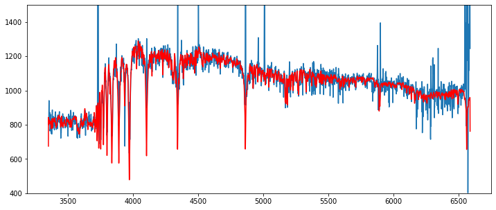
rescont = pf.fit_cont(sp, z, vdisp=80)
fig,ax = plt.subplots(1,1,figsize=(12,5))
tab = rescont['table_spec']
ax.plot(tab['RESTWL'],tab['FLUX'])
ax.plot(tab['RESTWL'],tab['CONT'], '-r')
ax.set_ylim(400,1500)

[51]:

(400.0, 1500.0)

[52]:

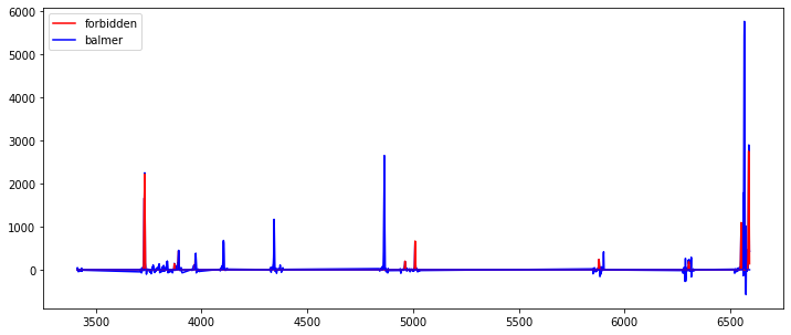
resline = pf.fit_lines(rescont['line_spec'], z)
fig,ax = plt.subplots(1,1,figsize=(12,5))
tab = resline['table_spec']
ax.plot(tab['RESTWL'],tab['FLUX'], '-b')
ax.plot(tab['RESTWL'],tab['FORBIDDEN_FIT_LSQ'], '-r', label='forbidden')
ax.plot(tab['RESTWL'],tab['BALMER_FIT_LSQ'], '-b', label='balmer')
ax.legend()

[52]:

<matplotlib.legend.Legend at 0x7fe36bf76ee0>

Output results in detail¶

The dictionary return by fit_spec contain the following items:

ztable: the redshift table (see fit_spec in the doc main menu for the meaning of table columns)
lines: the lines table (see fit_spec in the doc main menu for the meaning of table columns)
spec: the input spectrum
spec_fit: the full fit spectrum (cont_fit + line_fit + abs_fit)
cont_spec: the fitted model continuum + smooth low order residual spectrum
cont_fit: the fitted model continuum spectrum
line_spec: the emission line spectrum after subtraction of the fitted continuum (spec - cont_spec)
line_fit: the emission line fit spectrum
line_initfit: the initial solution for the emission line fit
abs_cont: the polynomial continuum fit spectrum
abs_init: the initial solution for the absorption fit (spec - abs_cont)
abs_fit: the fitted absorption lines spectrum
dline: dictionary with detailed results for the emission or absorption lines fit
dcont: dictionary with detailed results for the continuum fit

The dictionary dline contain the following items:

table_spec: rest frame emission line table data used in the fitting process
abs_table_spec: rest frame ansorption line table data used in the fitting process
lmfit_family: lmfit raw result with family, the family name.

The dictionary dcont contain the following items:

table_spec: rest frame flux table data used in the fitting process
success: boolean True if fit was successful
status: output fit message
z: metallicity for the best fit
ebv: E(B-V)
init_z: used redshift for the fit
chi2: \(\chi^2\) fit
ages: return list of ages for the model library
weights: returned list of weights for the model library

For example to display the detail lmfit result for the balmer family one can do (check lmfit for all the available info):

[53]:

sp = Spectrum(os.path.join(datadir, 'udf10_00002.fits'))
res = fit_spec(sp, z=0.41892)
res['dline']['lmfit_balmer']

[53]:

Fit Statistics

fitting method	least_squares
# function evals	7
# data points	783
# variables	11
chi-square	192511.056
reduced chi-square	249.366652
Akaike info crit.	4332.23974
Bayesian info crit.	4383.53420

Variables

name	value	standard error	relative error	initial value	min	max	vary
dv_balmer	82.1268012	3.85608873	(4.70%)	0	-500.000000	500.000000	True
vdisp_balmer	66.1085450	4.26045940	(6.44%)	50	5.00000000	300.000000	True
balmer_H11_gauss_l0	3771.69995	0.00000000	(0.00%)	3771.7	-inf	inf	False
balmer_H11_gauss_flux	196.541129	395.983771	(201.48%)	342.9287624503839	0.00000000	inf	True
balmer_H10_gauss_l0	3798.97998	0.00000000	(0.00%)	3798.98	-inf	inf	False
balmer_H10_gauss_flux	323.278214	384.247522	(118.86%)	343.22898429783106	0.00000000	inf	True
balmer_H9_gauss_l0	3836.46997	0.00000000	(0.00%)	3836.47	-inf	inf	False
balmer_H9_gauss_flux	573.322336	380.741042	(66.41%)	487.2757666583839	0.00000000	inf	True
balmer_H8_gauss_l0	3890.14990	0.00000000	(0.00%)	3890.15	-inf	inf	False
balmer_H8_gauss_flux	1302.15623	386.597943	(29.69%)	1106.9039675218417	0.00000000	inf	True
balmer_HEPSILON_gauss_l0	3971.19995	0.00000000	(0.00%)	3971.2	-inf	inf	False
balmer_HEPSILON_gauss_flux	1107.83505	378.329015	(34.15%)	944.1861023360569	0.00000000	inf	True
balmer_HDELTA_gauss_l0	4102.89014	0.00000000	(0.00%)	4102.89	-inf	inf	False
balmer_HDELTA_gauss_flux	2051.52603	379.267737	(18.49%)	1652.1183642247636	0.00000000	inf	True
balmer_HGAMMA_gauss_l0	4341.68018	0.00000000	(0.00%)	4341.68	-inf	inf	False
balmer_HGAMMA_gauss_flux	3647.93827	348.920115	(9.56%)	2994.6600370494198	0.00000000	inf	True
balmer_HBETA_gauss_l0	4862.68018	0.00000000	(0.00%)	4862.68	-inf	inf	False
balmer_HBETA_gauss_flux	8567.47174	415.428624	(4.85%)	7094.975428006051	0.00000000	inf	True
balmer_HALPHA_gauss_l0	6564.60986	0.00000000	(0.00%)	6564.61	-inf	inf	False
balmer_HALPHA_gauss_flux	23693.2431	2927.08919	(12.35%)	18925.797028608496	0.00000000	inf	True

Correlations (unreported correlations are < 0.100)

vdisp_balmer	balmer_HBETA_gauss_flux	0.3279
dv_balmer	balmer_HBETA_gauss_flux	0.2289
dv_balmer	balmer_HALPHA_gauss_flux	-0.2239
vdisp_balmer	balmer_HGAMMA_gauss_flux	0.2237
vdisp_balmer	balmer_HDELTA_gauss_flux	0.1048

[ ]:

[ ]: